Understanding Market Saturation: Why You Should Never Hesitate in Business

A new technology, culture shift, social phenomenon, or even a crisis can create a new market that could be potentially worth millions (or even billions) of dollars to your business. But how long it will last is purely a numbers game – one that doesn’t end well for the hesitant.

This article reveals truths about market saturation, and why market share is on a first-come, first-served basis.

What is Market Saturation?

A market is formed when there is a sudden need for a product or service that is sufficient enough to compel the forces of demand and supply to coexist in such a space, necessitating commercial exchange on the basis of price and quality.

When a market is created, the first to enter the market attracts a sizable portion of the market regardless of entry price (because the need for the product or service is so great). 

The market dynamics favor the initial entrant – until there is a new competitor.

The second entrant into the market will most likely enter with a lower price for a reasonably similar level of quality. The result? There will be sizable defections from the original demand enjoyed by the first entrant to the second, as well as new demand created purely by the introduction of the second entrant.

[Related Article: How to Figure Out Your Optimal Number of Business Outlets]

Things will now look rosy for the second entrant while the first entrant may suffer demand losses (but still retain market lead due to brand loyalty and large initial market capture). 

These conditions will only be reversed if the second entrant comes in with a higher price or significantly lower quality than the first (a faux pas). In which case, the second entrant will attract very little demand and the first entrant will attract even higher demand and more brand loyalty.

These scenarios are repeated when newer entrants penetrate the market – the only constant fact is that the actual market size available for new competitors reduces with each additional entrant into the market.

This happens until there is virtually no demand space left for a new entrant – a phenomenon known as market saturation.

Visualizing Market Saturation

Market saturation is as much a mathematical phenomenon as it is an economic phenomenon. With every new market entrant, the size of available demand for a new competitor becomes exponentially smaller with lower likelihood of profits.         

At the simplest level, market saturation is based on the following mathematical model:

The mathematical nature of market saturation means we can visualize it graphically and better understand why we need to act quickly when breaking our products and services into new or existing markets.

The graph below shows how market saturation works:

The graph shows a simulation for a market with 100 million subscribers. A very active market, the first entrant is able to whip up more than 40 million subscribers (40% market share) – and assuming 100% brand loyalty at this stage, this leaves only 60 million subscribers for any other new competitors to engage.

Realistically, the entrance of a second competitor would pull a portion of the first competitor’s demand, but overall, loyalty remains high and our model remains consistent.

The graph also shows that the second competitor enters the market, but is only able to pull in over 30 million subscribers (30% market share). Again, if we assume near-100% brand loyalty at this stage, this means the market is already 40% + 30% = 70% saturated, with only roughly 30% of the market up for grabs for any new competitor – this just after 2 entrants into the market.

Also bear in mind that the work new entrants have to do in order to capture demand from other camps increases with the increasing number of entrants into the market, because consumers start to adapt and normalize to currently available offerings (demand equilibration).

Statistical models show that most markets become saturated after only 5 competitors.

What does this mean for your business?

In short, it is never a good idea to enter a market late in the game. Always try to get in as early as possible to increase your chances of success.

Also, before launching a product, ensure that only a handful of major competitors exist. 

Entering a saturated market will render your product dead-on-arrival (DOA) unless you have some killer marketing strategy or something very special to offer that will help you win back some of the core demand lost to already established competitors.

A Simple and Free Forecasting Model for Your Small Business

If you run a small business, then you know how important it is to have an idea of what your monthly profits or sales may be, so you can plan ahead and better schedule your growth.

Thankfully, this is possible with tools such as forecasting. A business forecast studies the behavior of important business indicators like sales and expenses over long periods of time to arrive at a predictive model for future performance in those areas.

[Related Article: Modelling Important Business Decisions with Game Theory]

The validity of forecast models is guaranteed by the mathematical nature of business processes; your business can be modeled as a mathematical system receiving inputs (factors of production) and producing output (sales and profits).

Accuracy of forecast models is guaranteed by the fact that business performance fluctuates between reasonably fixed high and low points. 

These fluctuations may be seasonal (such as sales highs during holidays or profit lows in the first quarter of a new year), cyclic (consisting of alternating highs and lows), or reactive (consisting of nearly-random small changes). 

In any case, these fluctuations can be reasonably predicted over the long term using certain mathematical systems called forecast models. Software companies have successfully packaged these models into forecasting software that accurately predict key business performance indicators.

The problem is that many of these models are very complicated, and may not be suitable for relatively simple business processes – like those of small businesses. As a result of the complex nature of many of these programs, they are also very expensive. 

This post focuses on a simple and free forecast model for small businesses. 

Introducing the Mean Adjustment Prediction Model (MAPM) for sequential business data: 

With this model you can predict new monthly values of data given a substantial set of historical data by performing a simple calculation on a spreadsheet (e.g. MS Excel)

Read on to discover the actual equation for the model, as well as the code (formula) for EXCEL, so you can use this at home or in the office.

This forecast model is very simple and only requires that you obtain the mean (average) of the values of data you are interested in, and add an adjustment factor.

It is remarkable to note that this model does not sacrifice accuracy on account of its simplicity. For a detailed background of this model (open only if you are mathematically inclined), see Mean Adjustment Prediction.

For a simpler analysis, consider the following:

The MAPM is especially recommended for slightly-varying non-constant data, such as small business sales and profits.

Notice the high accuracy of the model (ranging between 87% and 120% for the example above). In the experiment shown above, MAPM was used to guess random sales figures ranging between $7,000 and $9,000 with very impressive results. Accuracy values in excess of 100% indicate an optimistic prediction (greater than the actual result).

Tip: I recommend you use MAPM in a spreadsheet to quickly calculate a prediction for applications such as planning and budgeting.

To use MAPM with Excel, you can use the following formula:

=AVERAGE(B3:G3) + 0.5*(G3 - B3)*(1 - 1/N)

B3 = first value in sequence

G3 = last value in sequence

N = number of values in sequence

I understand it’s a little technical, but I assure you it works great every time – and of course, it’s free. So by all means get started with MAPM in Excel and let me know if you need any assistance! Thanks for reading!

Winning Ways: Modeling Important Business Decisions with Game Theory

What do you do when you can’t quite figure out which of two strategies is best for your new business idea?

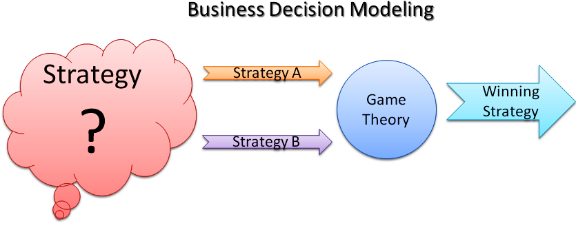
You simulate. Experts in economic modeling and business decision modeling recommend that you simulate your strategies before actually adopting them through game theory.

What is Game Theory?

No, game theory has nothing to do with video games or games you play with friends at the club house!

With game theory, businesses have a tool for making optimized guesses with respect to winning strategies for their products, services, or processes.

[Related Article: Understanding Market Saturation - Why You Should Never Hesitate]

How Do Business Games Work?

In a simple business game, you have two prospects, A and B. Consider the example below:

In this example, a business owner wants to decide between two prospects; either opening a new office (A) or expanding the current office (B) with the goal of generating the highest sales by the end of the year.

Case Study: Figuring Out Sales

To demonstrate game theory, we’re going to use the scenario described above as a case study. To move forward, we have to figure out how to arrive at a simple equation for sales. Don’t panic – it’s elementary:

Visibility

As shown above, we first describe your business’ visibility as the portion of the local population that is within your catchment factor. Catchment factor figures tend to be higher for products and services that are required daily or very frequently, as opposed to luxury or specialty products.

A reasonable catchment factor for a produce store can be 20% (adjusting for competition) while that for a luxury makeup store can be something like 3%.

So let’s say you run a produce store with a catchment factor of 20% in an area with a population of 10,000 people. Your visibility is 10000 x 20% = 2000 people. This means the maximum exposure for your business in that area is around 2,000 people.

Demand

Once you know your visibility, the next step is to figure out demand. What portion of your visible population is confident enough to buy your products or use your services? 

For the purpose of this case study, let’s keep the confidence factor at 20% (for a very credible and well-advertised business). This gives us a demand of 2000 x 20% = 400 people. This means you can expect to have about 400 regular customers year-in, year-out. This is your estimated fixed demand.

Daily Demand

Now you know your estimated fixed demand, the next question is: what portion of your fixed demand comes to your store daily? This is useful for simulation purposes. 

For this case study, which involves a produce company, it is reasonable that up to a quarter (25%) of the fixed demand will come to the store each day due to highly perishable goods. This is the daily factor. Daily demand in this case is therefore 400 x 25% = 100 people. This means 100 people visit the produce store each day.

Daily Sales

Figuring out the daily sales is easy at this point because every store owner knows the average quantity of items bought (per customer) per day and the average cost of items in the store. Your POS application and automated sales reports can probably tell you that.

Let’s say for this case study, the produce store sells an average of 5 items per customer per day, with an average cost of $10 for items in the store. Daily sales is simply 100 x 5 x 10 = $5,000 (per day).

Total Sales

This is simply the product of daily sales and the number of days we are considering. For a 30-day period, total sales in this case can be projected at 5000 x 30 = $150,000.

Simulation: Building Variables and Weighing the Prospects

Now that we have arrived at a convenient way of calculating sales, we then move on to the important task of evaluating two prospects (A and B) to see which generates higher sales over time.

To do this, we need to build models for each of the prospects. 

Modeling Prospect A: Opening a New Office

As shown above, we select the daily sales for the new office to vary between 20% and 80% of the current office sales because the current office is more established, and it has more dedicated customers. 

Modeling Prospect B: Expanding the Current Office + Advertising

For the second strategy (a mix of office expansion and advertising), we reasonably fix the expanded office sales at between 10% and 20% more sales daily compared to the current office. Additionally, we estimate that advertising will pull in an extra 2% to 10% more sales daily (for the expanded office).

It’s now time to simulate these two prospects over a large number of cycles or ‘games’ to determine which one pulls in the highest sales in the period under consideration. Let’s assume that the period of simulation is 6 months and the current daily sales is $5,000 as previously calculated.

Simulation Results: Produce Store Sales Strategy

A simple computer program was required to simulate the total period sales for prospects A and B. I created the program and ran this simulation for 10,000 cycles. Results are shown below:

Prospect A Sales ($, after 6 months)	Prospect B Sales ($, after 6 months)
1,349,586.82	1,096,734.11
1,348,620.29	1,096,658.02
1,348,884.86	1,096,665.31
1,347,971.19	1,096,760.43
1,349,250.91	1,096,743.23
1,348,760.7	1,096,785.42
1,348,480.92	1,096,705.68
1,349,177.55	1,096,750.2
1,348,943.75	1,096,730.62
1,348,972.28	1,096,784.42

Prospect A (opening up a new office) showed higher sales figures (approx. $1.348 million at the end of the period) than the option (prospect B) but lower long-term growth stability. This may mean that even though sales will be much higher in the short term, they will tend to stabilize or flatten at some point.

Prospect B (expanding current office and setting up advertising) showed lower sales figures (approx. $1.096 million at the end of the period) but higher long-term growth stability. Observe how the general trend of the sales figures is upwards as opposed to prospect A with a relatively stable-to-downward sales figure trend.

If the business owner uses prospect B as a strategy, s/he will experience higher long-term growth amidst lower short-run sales compared to prospect A.

This is the type of analysis and insight you get by using game theory to model your business decisions before making them.

I hope you enjoyed reading this article! If you have a question about simulation and game theory email me at montyblogger2014@gmail.com or just reply below with your comments!